
Reimagining Uber Freight’s carrier pricing algorithm to drive better outcomes
By: Kenneth Chong (Sr. Applied Scientist), Joon Ro (Sr. Applied Scientist), Emir Poyraz (Sr. Engineer) and May Wu (Applied Science Manager)
An innovative spin on a classic algorithm
Uber Freight operates a two-sided marketplace, which separately interfaces with shippers (who seek to move loads from point A to point B) and with carriers (truck drivers who move these loads). Both sides of this marketplace are powered by dynamic pricing algorithms. Each is structured a bit differently based on the needs of the respective marketplace.
Recently, our team identified the need to change the algorithm dictating carrier pricing. The algorithm generates a rate based on a variety of factors like market conditions, the size of the load, distance to move the load, etcetera. Up until this point, we used an algorithm based upon Markov Decision Processes (MDP) to set carrier prices (see this earlier blog post for a full description of how the MDP model works) because it is natural to our problem: we need to make pricing decisions sequentially over time. Over time, though, we realized that while the algorithm was performant, it had shortcomings that were challenging to address with a standard MDP implementation.
We overcame these by:
1) Truncating the backward induction
2) Relying more heavily on machine learning (ML) to approximate the value function
3) Developing a new clustering algorithm to identify “similar” loads that may be useful in estimating cost—creatively combining optimization and ML to develop what we think is a more robust version of MDP.
MDP is a natural choice of algorithm, but implementation is challenging
To briefly illustrate the problem of carrier pricing, suppose that we have made a commitment with the shipper to haul a load from Chicago, IL to Dallas, TX. The pickup appointment begins exactly 5 days from now: in other words, the lead timeT is 120 hours. Because it becomes more difficult to find carriers on shorter notice, prices tend to increase as lead time decreases. Thus, we have a sequence of decisions to make over time, which we refer to as a price trajectory:
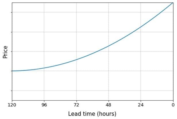
Figure 1: Example of a price trajectory over 5-day lead time
Because we update prices hourly, this trajectory can be represented as a sequence {pt}t{T, T-1, …, 0}, where pt is the price offered t hours from pickup. The goal of our algorithm is to pick a trajectory that minimizes, in expectation, the total cost to cover the load. We refer to this quantity as eCost:
eCostT=t=T0ptPr(Bt=1 | pt,St),
where Bt = 1 if load i is booked at lead time t (0 otherwise), and St denotes (possibly time-varying) state variables other than price that can affect the booking probability. This quantity usually increases as time passes and the load remains unbooked.
With MDP, computing eCost entails solving the Bellman equation
Vt =minptPr(Bt | pt, St)pt +1-Pr(Bt | pt, St)Vt-1 t{0, 1, …, T}
The quantities {Vt} are directly interpretable as eCost, conditional on our pricing policy. However, a crucial input into MDP is accurate estimates of the booking probabilities Pr(Bt=1 | pt , St). Although the ML model we use for this performs well, errors can compound over time. This means we become vulnerable to the optimizer’s curse, which states that in the presence of noise, total cost estimates associated with the optimal decision are likely to be understated. This, in turn, leads to lower, overly-optimistic prices that tend to decrease further at higher lead times.
In addition, the curse of dimensionality presents significant challenges in modeling more complex state transitions. For example, incorporating near-real-time (NRT) features, such as app activity, into our prices entails adding those to state variables – which quickly makes our problem computationally infeasible.
Our approach: carefully blending prediction and optimization
To improve pricing accuracy, we explored using a predictive model, rather than a standard backward induction, to estimate eCost. In particular, we perform K ≤ T stages of backward induction, and if the load remains unbooked after K hours, we substitute for the continuation value VT-K a prediction from this model. In this case, the Bellman equations become:
Vt =minptPr(Bt | pt, St)pt +1-Pr(Bt | pt, St)Vt-1 t{T-K+1, …, T-1, T}
with the boundary condition VT-K =eCostT-K.
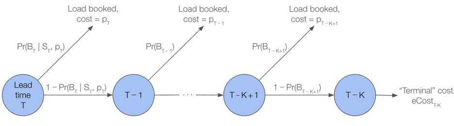
Figure 2: Illustration of sequential decision making in MDP
Picking an appropriate value for K required some iteration, but this truncated backward induction helps to mitigate each of the issues we highlighted above.
An initial candidate for such a predictive model was an XGBoost ensemble that we previously used elsewhere in carrier pricing. The training data consisted of historical loads, their characteristics (we describe these in more detail below), the lead times at which they were booked, as well as their realized costs.
However, the predictions generated by this model were not suitable for estimating eCost for two reasons.
There is an important distinction to be made between a load’s remaining lead time, and its available lead time. While we would include the former in the feature vector at time of serving, there are systematic patterns in the latter. That is, similar loads tend to become available at specific lead times. For example, longer hauls tend to become available with higher lead times than shorter hauls. Thus, we would have concentrations of data points around certain available lead times, making predictions at other lead times less reliable.
The training data consisted solely of outcomes—the realizations of random variables, rather than their expectations— so predictions from this model could also not be interpreted as an eCost. It was not clear how to modify the training set so that predictions from the XGBoost model could be treated as expectations
Instead of trying to predict eCost directly, we borrow principles from clustering to find a set of loads that are similar to the one to be priced, and take a weighted average of their total costs. With this approach, remaining lead times can be explicitly incorporated into eCost — we can exclude, from the set of similar loads, ones that were booked sooner than the remaining lead time of the current load. Moreover, each of the similar loads identified can be viewed as a potential outcome for the current load, which are assigned probabilities equal to the weights used in the averaging.
The primary challenge here is developing a way to measure similarity between loads, which we describe with a number of attributes:
Locations of the pickup and delivery facilities
Time of day, day of week the load is scheduled to be picked up or delivered
Market conditions around the time the load is scheduled to be moved
There is a mixture of continuous and categorical features, and it is not at all clear how these should be weighted against each other when computing similarity.
… with an unconventional clustering algorithm
We developed a new algorithm where our aforementioned XGBoost model is used to perform clustering. Consider the simple case where our model is a single (shallow) decision tree with a lone feature: driving distance. We might obtain a tree like the following:
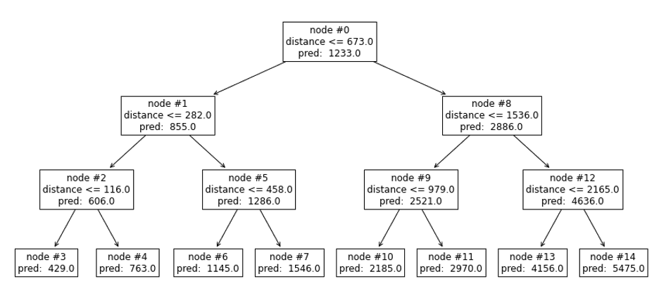
Figure 3: Illustration of a single decision tree for clustering
Two loads can be viewed as “similar” if their predictions are made from the same leaf node. In the case of leaf node #6, we know that their route distances are both between 282 and 458 miles.
This might seem like a crude way of measuring similarity, but by growing deeper decision trees and incorporating more features, we require the two loads to have comparable values on a number of dimensions to be considered “similar.” We can further differentiate by growing additional trees. In a nutshell, we associate with each load an embedding vector, consisting of nonzeros at locations matching with the leaf nodes the load falls into. We measure similarity between loads through the cosine similarity of their embeddings, which is directly related to the number of trees in which both have common leaf nodes.
Smoother prices led to improved booking outcomes
Given the fairly substantial changes we made to the algorithm, we performed a rollout in two main phases. First, we incorporated eCost into the algorithms we used in secondary booking channels, and conducted an A/B test to ensure no performance decline. Second, we ran a switchback experiment comparing it with the previous version of MDP. The net effect of these two experiments was a statistically significant reduction in the total cost of covering loads, without any negative impact on secondary metrics. We attribute this to the smoother price trajectories generated by the new algorithm, which results in loads being booked earlier in their lifecycles. This is particularly relevant, as costs tend to increase sharply once lead times fall below 24 hours.
With the rollout of this new algorithm comes a number of secondary benefits. The earlier booking of loads, due to smoother price trajectories, not only reduces costs but is crucial in avoiding the sharp cost increases associated with shorter lead times. Reducing the total cost to cover loads allows us to offer more competitive pricing to shippers— which, in turn, increases volume. Additionally, flatter price trajectories might lead to carriers checking loads on the app earlier in their life cycles. Beyond these business advantages, the algorithm has also contributed to reducing technical debt by unifying pricing across booking channels, as well as by removing nonessential components used in the previous implementation of MDP.
Though we think there are areas for further improvement, this new pricing algorithm provides a blueprint for how MDP can be applied to new use cases within Uber Freight.
*Since we are also using eCost as a sort of value function approximator, the problem we now solve shares some similarities with an approximate dynamic program.